Databases
Learn how databases organize data for fast retrieval, which storage engine to choose for your workload, and how ACID transactions keep concurrent writes correct at scale.
Introduction
A database combines three concerns that applications otherwise have to build themselves: efficient query execution, safe coordination of concurrent work, and durable recovery after failure. The useful design question is not simply which database is popular, but which data model, query shape, and correctness requirement the workload needs. Mental model: the planner chooses a route, the storage engine moves pages, and the transaction log makes committed state recoverable.
TL;DR
- A database is not just a place to store data — it is a query engine, a concurrency manager, and a durability mechanism packaged together. A defensible design accounts for all three layers.
- The storage engine (B-Tree vs. LSM-Tree) determines your read/write trade-off before you write a single query. B-Tree for balanced OLTP; LSM-Tree for write-heavy workloads where sequential I/O matters.
- Indexes are often the highest-leverage performance tool in a database. A missing index can turn a 1ms primary-key lookup into a 30-second full-table scan at 100M rows. A composite index in the wrong column order may provide little benefit.
- ACID (Atomicity, Consistency, Isolation, Durability) addresses four distinct failure and concurrency concerns. Each property has supporting mechanisms: transaction logging for atomicity and recovery,
fsyncfor durability, isolation levels for read/write anomalies, and constraints for data invariants. - The right database for a job is determined by your query shape — specifically, whether you need JOINs, which indexes you'll build, write vs. read ratio, and consistency requirements — not by your data format or team preference.
The Problem It Solves
It is Q4 earnings. Your fintech platform has processed 2 billion transactions this year. A risk analyst needs every transaction from account ACC-8841 in the last 90 days, grouped by merchant, filtered to amounts over $500.
Simple enough — except your transactions live in a distributed file system as individual JSON files, one file per transaction. Finding account ACC-8841's transactions means opening all 2 billion files sequentially. At 0.1ms per file open, that is 55 hours of I/O.
Meanwhile, your reconciliation service is reading existing transaction files while the payments service is writing new ones. No locking. A payment file half-written by the payments service is read mid-write by the reconciliation service.
The reconciliation total is wrong — but by how much? There is no way to know. The file system does not track partial writes.
And at 2:47 a.m., your transaction processing server crashes between writing the debit record and the credit record. Alice's $200 was debited. Bob never received it.
This failure mode may remain hidden until a customer or reconciliation process reports a missing transfer. Without a transaction log or rollback semantics, it is difficult to know which transfers completed and which are half-done.
The 'we can figure out schema later' trap
Raw files and key-value stores feel fast to build with early on. They collapse under three specific pressures: multi-column query patterns (you can only index what you anticipated), concurrent writes without coordination (race conditions that only appear under load), and crash recovery (the question becomes "how much data did we lose?" not "did we lose any?"). Every database exists to solve these three problems simultaneously.
A database solves all three failure modes in a single system: it gives you indexes for fast queries, transactions for concurrency safety, and a write-ahead log for crash recovery. These aren't nice-to-haves — they're the reason databases exist.
What Is It?
A database is a structured data store with three integrated subsystems: a query interface that translates your intent into an execution plan, a storage engine that physically organises data for the access patterns you need, and a transaction manager that serialises concurrent operations and ensures committed changes survive failures. Understanding all three subsystems makes storage trade-offs easier to reason about.
Analogy: Think of a large reference library with millions of books. If books were stored at random, finding all books published in 1987 on quantum physics requires reading every title. A library solves this with a card catalogue (B-Tree index), books shelved by subject and author (storage model), a sign-out ledger (transaction log), and a fireproof copy of the catalogue offsite (durability).
The catalogue is not the library — it is the structure that makes the library useful at scale. Your schema, indexes, and access patterns are the catalogue.
With a database, the risk analyst's query becomes:
SELECT merchant_id, SUM(amount), COUNT(*)
FROM transactions
WHERE account_id = 'ACC-8841'
  AND created_at >= NOW() - INTERVAL '90 days'
  AND amount > 500
GROUP BY merchant_id
ORDER BY SUM(amount) DESC;
With a composite index on (account_id, created_at, amount), this can execute in a few milliseconds on a warm, selective index, even when the table is much larger — because the storage engine traverses the B-Tree to account ACC-8841, range-scans the last 90 days, and filters the rest. It avoids rows for other accounts. The exact latency depends on data distribution, cache state, hardware, and the planner's chosen plan.
How It Works
Here is what happens end-to-end when your application issues SELECT * FROM products WHERE id = 7429:
- Connection pool assigns a connection — Your application maintains a pool of persistent database connections. A new request borrows one instead of negotiating a full TCP + auth handshake (5–50ms overhead per request without a pool).
- Parser validates syntax — The SQL string is tokenised and parsed into an Abstract Syntax Tree. Syntax errors are caught here before touching any data.
- Query planner chooses an execution plan — The planner checks
pg_statisticsfor row count estimates, index availability, and selectivity. Ifidis a primary key (clustered B-Tree index), the plan is:Index Scan using products_pkey on products WHERE id = 7429. If no index exists:Seq Scan on products— read every row. - Execution engine runs the plan — For an index scan, it traverses the B-Tree from the root to the leaf page containing
id = 7429. - Buffer pool check — Before hitting disk, the execution engine checks the in-memory buffer pool. If the page is already cached (~95% hit rate on hot data), it returns immediately (< 0.5ms). On a miss, it fetches the 8KB page from disk (~1–5ms SSD, ~5–15ms HDD) and warms the buffer pool for future access.
- Result returned — The deserialized row data is returned to the connection and ultimately to your application.
// Application layer — always use parameterised queries (prevents SQL injection)
async function getProduct(productId: number): Promise<Product | null> {
  // Connection pool handles connection acquisition; do NOT create one per request
  const result = await db.query<Product>(
    'SELECT id, name, price, stock_qty FROM products WHERE id = $1',
    [productId]  // Parameter, not string interpolation — prevents SQL injection
  );
  return result.rows[0] ?? null;
}
-- Debug slow queries with EXPLAIN ANALYZE (PostgreSQL)
EXPLAIN ANALYZE
SELECT id, name, price FROM products WHERE id = 7429;

-- Without index (catastrophic at 100M rows):
-- Seq Scan on products  (cost=0.00..2843291.00 rows=1 width=40)
--   (actual time=28943.871..28943.872 rows=1 loops=1)
-- Planning: 3.2ms · Execution: 28943.9ms (29 seconds!)

-- With primary key index (default B-Tree):
-- Index Scan using products_pkey  (cost=0.56..8.58 rows=1 width=40)
--   (actual time=0.042..0.043 rows=1 loops=1)
-- Planning: 0.1ms · Execution: 0.043ms (instant!)
Measure before adding infrastructure
For a slow query, start with EXPLAIN ANALYZE to confirm the execution plan. A missing or poorly ordered index, an unselective predicate, a bad join order, or an N+1 access pattern may be cheaper to fix than adding a cache or another database tier.
The sequence from query to data on every non-trivial request:
Key Vocabulary and Components
| Component | Role |
|---|---|
| Query parser | Converts SQL string into an Abstract Syntax Tree. Rejects malformed queries immediately. |
| Query planner / optimiser | Chooses the execution plan: which indexes to use, join ordering, predicate pushdown. Wrong plans are the leading cause of unexplained slowdowns. |
| Execution engine | Runs the plan: iterates rows, evaluates predicates, aggregates results. For complex queries, this stage does the most CPU work. |
| Buffer pool | In-memory cache of disk pages (typically 25–80% of RAM in PostgreSQL). The goal is a 95%+ hit rate so most reads never touch disk. The database equivalent of an application-level cache — but automatic. |
| Storage engine | Manages the on-disk layout: B-Tree for PostgreSQL/MySQL, LSM-Tree for Cassandra/RocksDB. Determines read/write performance characteristics. |
| Write-Ahead Log (WAL) | Every write is appended to the WAL before touching data files. On crash, the DB replays the WAL to restore the committed state. This is how durability (the D in ACID) is implemented. |
| Transaction manager | Assigns transaction IDs, tracks in-flight transactions, enforces isolation levels, coordinates commits and rollbacks. Maintains MVCC snapshots. |
| Connection pool | Manages a pool of persistent DB connections. Creating a new connection costs 5–50ms and requires authentication + session setup. At 10K req/s, new-connection-per-request adds 50–500ms of pure overhead. |
| Replication slot | Tracks how far each replica has consumed the WAL stream. A lagging replica with a stale slot will prevent the primary from cleaning old WAL segments — a disk-space trap. |
| MVCC (Multi-Version Concurrency Control) | Maintains multiple row versions so readers never block writers. Readers see a consistent snapshot; they do not acquire locks. This is why PostgreSQL reads scale independently of writes. |
Storage Engines: B-Tree vs. LSM-Tree
The storage engine is the component that physically organises your data on disk. Choosing one that does not fit the workload can be expensive to change because it affects schema design, operational runbooks, and hardware needs. A statement such as "Cassandra scales better" is not an analysis without a write pattern, query shape, and target SLO.
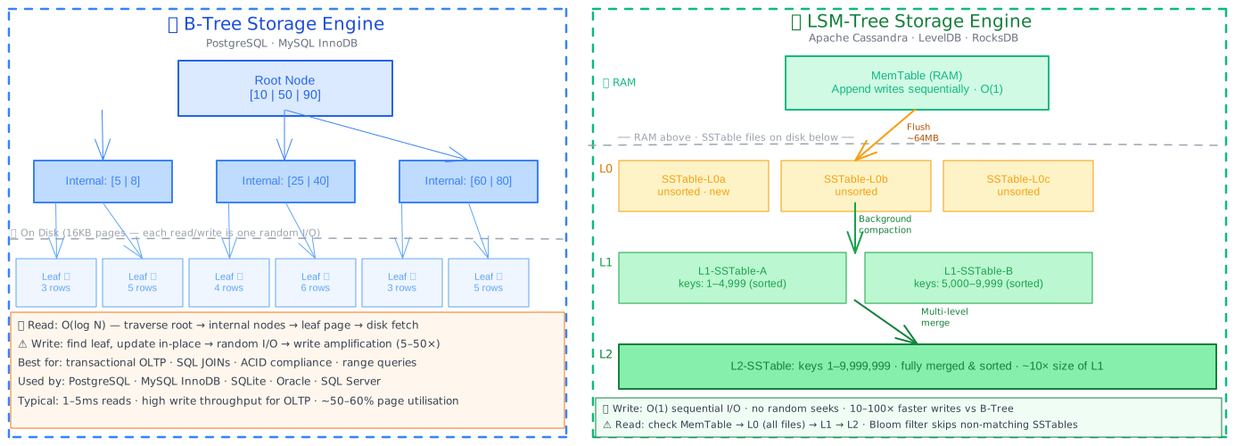
B-Tree
B-Trees store data as a balanced tree of fixed-size pages (typically 8KB). Every read and write traverses from the root to a leaf page.
The leaf pages contain the actual row data (or row pointers in a secondary index). Leaves are linked for efficient range scans.
Why it dominates OLTP: B-Tree provides O(log N) for both reads and writes, predictable latency, and efficient range queries (BETWEEN, ORDER BY, >, <). The standard page size means the OS page cache and the DB buffer pool interact cleanly, and SSD random read latency (0.1ms) is fast enough for typical OLTP query depths of 3–5 levels.
The write amplification problem: A single 100-byte row write may trigger an 8KB page rewrite. More critically, as the tree rebalances, a single insert near a full page triggers a page split: the existing page is copied, split into two new pages, and the parent page is updated. In heavy insert workloads, write amplification factors of 5–50× are common — one logical write becomes 5–50 physical disk writes.
LSM-Tree
LSM-Trees (Log-Structured Merge Trees) never update data in-place. All writes go to an in-memory buffer (MemTable) first. When the MemTable fills (~64MB), it is flushed as an immutable sorted file (SSTable) to disk.
Background compaction merges SSTables from Level 0 into larger sorted runs at Level 1, then Level 2, reducing the number of files reads must check.
Why it dominates write-heavy workloads: Writes are always sequential appends (O(1), no random I/O). On modern SSDs, sequential write throughput is 5–10× faster than random writes. This makes LSM-Trees ideal for time-series, IoT telemetry, event logs, and write-heavy analytics.
The read amplification problem: To find a key, the DB must check: MemTable → L0 (every file, since they're unsorted at L0) → L1 → L2 → … each additional level adds disk accesses. LSM-Trees use per-SSTable Bloom filters to skip files that definitely do not contain a key, but reads still hit multiple files vs. a single B-Tree path.
| Dimension | B-Tree | LSM-Tree |
|---|---|---|
| Write pattern | Random I/O — in-place update | Sequential I/O — always append |
| Write amplification | 5–50× (page splits, rebalancing) | 10–30× (compaction rewrites) |
| Read performance | O(log N) — single tree path | O(log N) with amplification — multi-level check |
| Range scans | Excellent — linked leaf pages | Moderate — must merge-read SSTables |
| Space efficiency | ~50–60% page utilisation | Higher — but compaction reclaims space |
| Compaction cost | None (tree maintains itself) | Background CPU/IO — can spike under heavy write load |
| Best for | OLTP · mixed read/write · ACID transactions | Write-heavy ingestion · time-series · analytics |
| Engines | PostgreSQL, MySQL InnoDB, SQLite, Oracle | Cassandra, LevelDB, RocksDB, ClickHouse (partial) |
The fundamental tension: read amplification vs. write amplification. B-Tree minimises read amplification (single path from root to leaf) at the cost of write amplification. LSM-Tree minimises write amplification (append-only) at the cost of read amplification (multiple levels to check).
Default to B-Tree unless your write throughput or append-only access pattern specifically justifies the LSM-Tree trade-off.
Indexing
An index is a separate data structure (usually a B-Tree) that stores a sorted subset of your columns with pointers back to the full rows. The query planner uses it to jump directly to relevant rows instead of scanning every row in the table. It is often the highest-leverage first step for a selective query, provided the index matches the access pattern.
Without an index on email: Find the user with email = 'alice@example.com' from 100M users → Full Table Scan → read every row → ~30 seconds.
With a B-Tree index on email: The planner traverses the B-Tree (5 levels deep at 100M rows) → jumps to the leaf page → fetches the row pointer → one disk I/O → < 1ms.
The 30,000× difference is possible in this example, but actual gains depend on selectivity, cache state, storage, and the query plan. Benchmark representative data rather than assuming a fixed multiplier.
-- See what the planner is doing
EXPLAIN ANALYZE SELECT * FROM users WHERE email = 'alice@example.com';

-- After adding index:
CREATE INDEX idx_users_email ON users(email);
-- Index Scan using idx_users_email on users
-- (actual time=0.041..0.042 rows=1 loops=1)  -- 0.042ms

-- Composite index: column order matters enormously
-- Query: WHERE account_id = 'ACC-8841' AND created_at >= '2026-01-01' AND amount > 500
CREATE INDEX idx_txns_account_date_amount
  ON transactions(account_id, created_at, amount);
-- The planner uses this index for the above query.
-- Index on (created_at, account_id, amount) would NOT use the account_id push-down —
-- range scan on the first column exhausts the index's selectivity benefit.
Index types
| Type | Data structure | Query support | Notes |
|---|---|---|---|
| B-Tree (default) | Balanced tree | Equality, range, LIKE 'prefix%' | 99% of indexes you will ever create |
| Hash | Hash map | Equality only — = | Faster than B-Tree for pure equality at the cost of range support |
| GIN/GiST | Inverted/spatial | Full-text search, arrays, JSON containment, geographic | PostgreSQL-specific; essential for @>, @@, && operators |
| Partial | B-Tree on filtered subset | Equality + range on the subset | CREATE INDEX ... WHERE status = 'active' — smaller, faster |
| Covering | B-Tree storing non-key columns | Index-only scan — zero table access | CREATE INDEX ... INCLUDE (price, stock_qty) |
| Composite | B-Tree on N columns | Left-prefix rule — first N columns must match | Column order matters: high-cardinality, equality-first columns first |
The left-prefix rule and when composite indexes fail
A composite index on (account_id, created_at, amount) is used by queries that filter on account_id, or account_id + created_at, or all three. It is NOT used by queries that only filter on created_at or amount alone — the first column must be constrained. Build composite indexes starting with the highest-cardinality equality column (usually an ID), followed by range columns, followed by low-cardinality filters.
Covering indexes — eliminating table access entirely
A covering index stores non-key columns directly in the index leaf pages. If all columns your query touches are in the index, the DB never fetches the underlying table pages — the query executes entirely from the index, which is typically much smaller and more cache-friendly.
-- Without covering index: index scan + heap fetch (table access)
CREATE INDEX idx_products_status ON products(status);
SELECT id, name, price FROM products WHERE status = 'active';
-- Plan: Index Scan → for each matching id, fetch the heap page for name + price

-- With covering index: index-only scan
CREATE INDEX idx_products_status_covering ON products(status) INCLUDE (name, price);
SELECT id, name, price FROM products WHERE status = 'active';
-- Plan: Index Only Scan — name and price come from the index, no table fetch
-- Typically 3–5× faster for wide tables with narrow query projections
The N+1 query problem
The most common application-layer database performance issue. Your ORM executes one query to fetch a list, then one query per item to fetch a related record.
// N+1 — catastrophic at scale
const orders = await db.query('SELECT * FROM orders WHERE status = $1', ['pending']);
// Returns 1,000 orders — then fires 1,000 individual queries:
for (const order of orders) {
  order.customer = await db.query(
    'SELECT * FROM customers WHERE id = $1', [order.customer_id]
  );
}
// Total: 1,001 queries · 1,000 round-trips · ~5 seconds for what should be 5ms

// Fix: JOIN or batched IN clause
const orders = await db.query(`
  SELECT o.*, c.name, c.email
  FROM orders o
  JOIN customers c ON c.id = o.customer_id
  WHERE o.status = $1
`, ['pending']);
// Total: 1 query · 1 round-trip · ~5ms ✅
Common slow-query causes include a missing index, the wrong composite-index column order, an unselective predicate, or N+1 access in the ORM layer — check these before adding caching or a new database tier.
Transactions and ACID
A transaction is a unit of work that either completes entirely or not at all. ACID describes what that means under failure and concurrency. A useful way to learn the four properties is through their implementation mechanisms — the WAL supports atomicity and recovery, fsync supports durability, MVCC supports snapshot-based isolation, and constraints help enforce consistency — rather than memorising the acronym alone.
The canonical bank transfer example — without transactions:
-- Session 1 executes these two statements independently (no transaction):
UPDATE accounts SET balance = balance - 100 WHERE id = 'alice';
-- ↑ Server crashes here (power failure, OOM, reboot)
UPDATE accounts SET balance = balance + 100 WHERE id = 'bob';
-- This line never executes. alice's $100 has vanished from the system.
With a transaction (ACID):
BEGIN;
  UPDATE accounts SET balance = balance - 100 WHERE id = 'alice';
  -- If server crashes here, WAL records the in-progress transaction.
  -- On restart, PostgreSQL sees an uncommitted transaction and rolls it back.
  -- alice's balance is restored. No money is lost.
  UPDATE accounts SET balance = balance + 100 WHERE id = 'bob';
COMMIT;
-- Only COMMIT makes the change permanent and visible to other sessions.
A — Atomicity
All operations in a transaction succeed, or none of them take effect. Implemented via the Write-Ahead Log (WAL): every change is logged before being applied. On crash, uncommitted changes are rolled back by replaying the WAL in reverse.
C — Consistency
A transaction can only bring the database from one valid state to another. Constraints, foreign keys, and check constraints enforce this: if any constraint is violated mid-transaction, the entire transaction is rolled back. Consistency is enforced by your schema design — the DB provides the mechanism.
I — Isolation
Concurrent transactions do not observe each other's intermediate state. Isolation levels control the trade-off between correctness guarantees and throughput:
| Isolation Level | Dirty Read | Non-Repeatable Read | Phantom Read | Performance |
|---|---|---|---|---|
| Read Uncommitted | ❌ Possible | ❌ Possible | ❌ Possible | ⚡⚡⚡ Highest |
| Read Committed (PostgreSQL default) | ✅ Prevented | ❌ Possible | ❌ Possible | ⚡⚡ High |
| Repeatable Read | ✅ Prevented | ✅ Prevented | ✅ Prevented (PostgreSQL MVCC) | ⚡ Moderate |
| Serializable | ✅ Prevented | ✅ Prevented | ✅ Prevented | 🐢 Lowest |
- Dirty read: Reading a row modified by an uncommitted transaction. Prevented by any level above Read Uncommitted.
- Non-repeatable read: Re-reading the same row within a transaction and seeing a different value (another transaction committed a change between your two reads).
- Phantom read: Re-running a range query and seeing new rows (another transaction inserted matching rows between your two queries).
Choose isolation from the invariant
PostgreSQL defaults to Read Committed because it prevents dirty reads while keeping throughput high. Use row locks, conditional updates, or Serializable isolation when the invariant requires the read-and-modify decision to be coordinated, such as financial double-spend prevention or inventory allocation. The right mechanism depends on transaction scope and contention.
D — Durability
A committed transaction survives server crashes, power failures, and hardware faults. Implemented by fsync: PostgreSQL calls fsync() on the WAL file before acknowledging COMMIT to the client. This forces the OS to flush the WAL to physical disk rather than retaining it in the OS page cache (which would be lost on a crash).
-- PostgreSQL synchronous commit settings (trade durability for throughput)
-- synchronous_commit = on   → fsync on every COMMIT (default, fully durable)
-- synchronous_commit = off  → async commit, ~10ms durability window (risk: last 10ms of commits lost on crash)
-- synchronous_commit = remote_write → commit when at least one standby has received the WAL
Get the WAL and MVCC mental models solid — every question about concurrent writes, replica lag, or crash recovery traces back to one of them.
Database Types
| Type | Data Model | Primary Access Pattern | Horizontal Scale | ACID | Examples |
|---|---|---|---|---|---|
| Relational | Tables with rows + fixed schema | Multi-column queries, JOINs, aggregations | Vertical + read replicas (sharding is manual) | Full | PostgreSQL, MySQL, SQLite |
| Document | Semi-structured JSON documents | Fetch document by ID or field; no JOINs | Native horizontal sharding | Per-document | MongoDB, CouchDB, Firestore |
| Key-Value | Opaque value per key | Single-key lookup only (no secondary index natively) | Horizontal sharding by key | Limited | Redis, DynamoDB, etcd |
| Wide-Column | Rows with sparse, dynamic columns | Key + column family lookup; append-optimised | Native horizontal sharding across nodes | Eventual/configurable | Cassandra, HBase, ScyllaDB |
| Time-Series | Timestamped metrics + tags | Range queries over time, downsampling, retention | Horizontal by time range | Limited | InfluxDB, TimescaleDB, Prometheus |
| Graph | Nodes + directed/labelled relationships | Relationship traversal (depth-first, shortest path) | Limited (JOINs are O(1) per hop) | Full (Neo4j) | Neo4j, Amazon Neptune, DGraph |
Which to choose and when
A common starting point is Relational, and a specific query shape or throughput requirement should justify moving to another model.
Relational is often a strong starting point for a new service when relationships, transactions, or varied query patterns matter. The useful question is not simply "can I use Postgres?" but "what query patterns does the chosen relational design make expensive?"
Document can fit when data is naturally hierarchical (for example, a blog post with nested comments) and the document is the primary access unit. Cross-document queries are still possible in some systems, but if they dominate the workload, a relational model or a separate read model may be simpler.
Wide-Column (Cassandra) can fit when write volume exceeds what a primary database can absorb, data is append-oriented, and read patterns are known and fixed to partition key plus clustering columns. Its strength is linear scale for that access pattern; its limitation is that queries outside the primary and clustering keys usually require denormalization or secondary indexes that can be expensive at scale.
Key-Value fits when the access pattern is primarily get(key) and set(key, value) — sessions, leaderboards, feature flags, or coordination state. DynamoDB adds secondary indexes and range queries on a sort key; Redis adds data structures such as sorted sets, streams, and pub/sub.
Time-Series is correct when your schema is (timestamp, metric_name, value, tags[]) and your queries are "average CPU over last 5 minutes, grouped by host". Time-series databases optimise for exactly this: they compress timestamp data aggressively, automatically downsample old data (replace per-minute points with per-hour averages after 30 days), and enforce retention policies that would require manual partitioning in PostgreSQL.
Polyglot persistence — using multiple databases in one system
Large-scale systems routinely combine database types for different workloads within the same product. Stripe uses PostgreSQL for transactional ledger entries, Redis for rate limiting and distributed locks, and a column store for analytics. This is called polyglot persistence and it is the correct architectural pattern — each database is used for what it does best, not everything.
The companies doing polyglot persistence earned it by starting simple and migrating to each database only when a specific pain point demanded it. Nobody wins by starting with four databases.
Failure Modes, Operational Concerns, and Trade-offs
Operational database failures usually come from a mismatch between the access pattern and the schema, an unbounded resource such as connections or dead tuples, or a correctness assumption that the isolation level does not provide. Measure query plans, lock waits, connection use, WAL/replica lag, cache pressure, and maintenance health.
| Pros | Cons |
|---|---|
| Indexes can reduce query time by 100–100,000× for selective lookups vs. full scans | Indexes add write overhead on every INSERT/UPDATE/DELETE — each index is a separate B-Tree that must be maintained |
| ACID transactions prevent data corruption under concurrent writes and crashes | Serializable isolation reduces throughput; every additional isolation guarantee costs concurrency |
| Relational schemas can enforce data integrity at the DB layer when constraints are defined | Schema migrations on large tables are expensive operations; ALTER TABLE ADD COLUMN on a 100M-row table can lock the table for minutes |
| Buffer pool caches hot pages automatically — most reads never hit disk | Buffer pool pressure from infrequent scans (OLAP queries) evicts hot pages needed by OLTP queries — mixed workloads conflict |
| Replication provides read scaling and high availability at low latency overhead | Replica lag introduces read-after-write inconsistency — a user writes a row, reads it back immediately from a replica, and it isn't there yet |
| PostgreSQL may handle 10K–50K transactional queries/second on modern hardware, depending on the workload | Horizontal write scaling requires manual sharding in relational databases — not a knob you turn, a re-architecture project |
| Mature tooling: pgvector, PostGIS, full-text search, JSONB, partitioning — all without leaving the relational model | Auto-vacuuming and dead tuple bloat in MVCC databases require operational discipline; a neglected table grows unboundedly until vacuum reclaims space |
The fundamental tension here is consistency vs. throughput. Each ACID guarantee restricts the concurrency model: Serializable isolation provides a serial execution view but can reduce the number of concurrent transactions the database can handle.
Every time you relax an isolation level or use eventual consistency, you trade a specific correctness guarantee for a specific throughput gain. The engineering discipline is knowing which anomalies are acceptable for each data type in your system.
When to Use It / When to Avoid It
The database choice matters whenever persisted state has meaningful query, correctness, latency, or scaling requirements. The data model determines query flexibility, consistency guarantees, and the scaling work required later.
Use a relational database (PostgreSQL) as your starting point when:
- Your data has relationships between entities that you'll JOIN — orders with customers, users with roles, payments with accounts.
- You need ACID transactions — financial operations, inventory management, any workflow where partial completion is incorrect.
- Your query patterns are varied and not yet fixed — relational indexes can be added after launch; a key-value schema cannot be retroactively queried.
- You are at < 10K writes/second on a single-tenant service. PostgreSQL handles this comfortably without sharding.
- Your team knows SQL. The operational cost of operating an unfamiliar database under production pressure is often higher than the cost of vertically scaling a familiar one.
Upgrade to a different database type when:
- Write throughput exceeds what a primary + N replicas can sustain → Wide-Column (Cassandra) or a queue-backed writes pattern.
- You are storing 100B+ time-stamped metrics with downsampling and retention requirements → TimescaleDB or InfluxDB.
- Your primary query is relationship traversal ("all friends-of-friends within 3 hops") → Graph database; this becomes exponentially expensive in SQL JOINs.
- Your schema is genuinely unknown and changes per customer (SaaS with per-customer custom fields at scale) → Document database, but validate that you truly never need cross-document queries before committing.
Avoid over-engineering by:
- Not choosing a NoSQL database because it "scales better" — define what scale you need and verify your chosen database cannot reach it before switching.
- Not sharding before you've exhausted read replicas, connection pooling, and query optimisation — sharding is a complexity multiplier that makes every future feature harder.
- Not using multiple database types before exhausting what your single database type can do with proper schema design (JSONB in PostgreSQL handles many document use cases with full SQL queryability).
Real-World Examples
The most instructive examples aren't the "we switched to NoSQL" stories — they're the "we stayed on PostgreSQL and here's exactly how" ones. The three below show what database discipline actually looks like at scale.
Stripe — PostgreSQL at financial scale
Stripe runs one of the largest PostgreSQL deployments in the world, processing hundreds of billions of dollars annually. Their key architectural decisions: every service owns its own isolated PostgreSQL instance (not a shared mega-DB), tables are partitioned by created_at and id so old partitions become append-only and can be archived to cold storage, and all financial mutations use serializable isolation to prevent double-processing.
Stripe does not use NoSQL for their core ledger — the correctness guarantees of relational ACID transactions are non-negotiable for payment data. Their scaling technique is not sharding; it is aggressive partitioning, careful index design, and splitting read-heavy operations onto read replicas.
Discord — 1 trillion messages: Cassandra → ScyllaDB migration
Discord stored their message history in Apache Cassandra. At 1 trillion messages, read latency became unpredictable: Cassandra's garbage collection pauses caused p99 read latency to spike from 5ms to 500ms under load. In 2023, Discord migrated to ScyllaDB (a Cassandra-compatible, C++-rewritten engine with lower GC overhead).
The migration achieved 99th percentile read latency drop from ~500ms to ~15ms on the same data and access patterns. The lesson: the data model (wide-column, partition by channel_id + bucket_id) was correct. The JVM garbage collector was the bottleneck, not the storage engine.
Notion — PostgreSQL at document-scale
Notion stores all workspace content in PostgreSQL. At 100M+ blocks across millions of workspaces, they use a physically partitioned schema: each customer workspace's data lives in separate PostgreSQL table partitions.
This keeps operational data access patterns local (no cross-workspace queries) and enables per-workspace backup, restore, and isolation. Notion deliberately chose PostgreSQL over a document database (despite storing JSON-like block structures) because of ACID transaction guarantees when a user edits a page simultaneously from multiple devices — the relational transaction model handles concurrent edits correctly; eventual-consistency document databases would require application-layer conflict resolution.
The pattern across all three: the bottleneck was operational or implementation-level, not a fundamental flaw in the core data model choice.
30-Second Explanation and 5-Minute Explanation
30-second explanation
A database combines query execution, durable storage, and concurrency control. Start with the query shapes and invariants: choose a data model and indexes that support the reads, a storage engine that fits the write/read pattern, and transaction semantics that keep valid state valid. Scale with measurement — query plans, connection pools, replicas, partitioning, and only then sharding or a different database type.
5-minute explanation
First describe the data model and the operations that matter: point lookups, ranges, joins, aggregates, relationship traversals, or append-heavy writes. Then explain how the planner uses indexes, how the storage engine reads or writes pages, and how the buffer pool and WAL affect latency and recovery. For concurrent changes, name the invariant and choose an isolation or conditional-update strategy; for cross-service workflows, use local transactions plus durable events and compensating actions when a Saga is appropriate. Finally, state the operational limits: connections, lock waits, WAL and replica lag, vacuum/bloat, migrations, and the read/write SLOs that trigger the next scaling step.
State a concrete database choice
Name the primary database with a rationale tied to the workload: for example, PostgreSQL for user and payment data when relational queries and ACID transactions matter, plus read replicas for read scaling. Introduce another database only when a specific query shape, retention policy, or throughput requirement is not served efficiently by the current design.
Database choices are sticky
Migrating a production database can be expensive because schema, access patterns, data pipelines, and operational runbooks are coupled to it. A new database should have a measurable reason to exist, such as a query shape or throughput/retention requirement that the current design cannot meet economically.
Practical questions and answers
- A single PostgreSQL primary may handle 10K–50K OLTP queries/second depending on schema, hardware, and query shape. PgBouncer can multiplex many application connections over a smaller database pool, and each replica adds read capacity only if the workload can tolerate replica lag.
- For a feed query, a composite index such as
(user_id, created_at DESC)puts the equality predicate first and the ordering/range dimension after it;INCLUDEcolumns may make it covering. - Read Committed prevents dirty reads but allows non-repeatable reads. Payment or inventory invariants may need a conditional update, row lock, or Serializable isolation.
- Shard only after query optimisation, pooling, vertical scaling, and read replicas are understood and insufficient. A key such as
user_idis useful only when it keeps common queries local. - Monitor vacuum/bloat, connection use, lock waits, WAL, and replica lag as part of the database's operating envelope.
| Question | Concise answer |
|---|---|
| "How do you handle 300K writes/second?" | "That's beyond a single PostgreSQL primary (~50K w/s). I'd evaluate: (1) can writes be made async via a queue? (2) can the write table be sharded by user_id? (3) is the write pattern time-series (→ Cassandra/LSM-Tree)? Before choosing, I need to know if writes are idempotent and whether ORDER BY queries across all writers are required." |
| "What happens to reads when you add a read replica?" | "Reads on the replica see replica lag — typically 10–200ms behind the primary. For read-after-write (user posts a comment and immediately sees it), route the read back to the primary for that session. For analytics and reporting queries, replica lag is acceptable. Alert if replica lag exceeds your SLA threshold — aggressive vacuum or large transactions on the primary cause it." |
| "How does PostgreSQL handle concurrent updates to the same row?" | "MVCC: readers never block writers. Writers queue behind each other per row via row-level locks (SELECT FOR UPDATE). PostgreSQL uses optimistic concurrency for reads: each transaction gets a snapshot; if two writes conflict, the second writer's transaction is aborted and must retry. This is why application retry logic on serialization_failure errors is required." |
| "When would you choose MongoDB over PostgreSQL?" | "When the data is genuinely document-shaped, schema evolution is rapid, documents are the primary access unit, and the scaling or operational requirements justify it. Evaluate MongoDB's transaction and consistency settings for multi-document operations; PostgreSQL with JSONB handles many document-like schemas with full SQL queryability." |
| "How do you prevent an expensive OLAP query from killing your OLTP latency?" | "Query isolation: route OLAP queries to a dedicated read replica or a Redshift/BigQuery analytical store. On the OLAP replica, configure statement_timeout to kill runaway queries before they consume all connections. Physically separate OLAP and OLTP workloads at the hardware level — they have opposite profiles (OLAP: sequential I/O, many rows, low concurrency; OLTP: random I/O, few rows, high concurrency)." |
Trace each trade-off to a mechanism — for example, row-level locks serialize conflicting writes, while Serializable isolation adds validation or coordination that can reduce throughput.
Common Mistakes and Misconceptions
- Choosing by database brand or data format. Start with query shapes, relationships, write/read ratios, consistency requirements, and retention before choosing a product.
- Adding single-column indexes without checking the plan. Low-cardinality indexes may be ignored, and composite indexes depend on column order and the left-prefix rule.
- Assuming ACID or Read Committed solves every race. A check followed by an update still needs a conditional write, row lock, or an isolation level that covers the invariant.
- Treating connections as free parallelism. A connection pool limits active database work; thousands of idle backend connections consume memory and can exhaust the database before throughput improves.
- Using a cache or Redis counter as the durable source by accident. Define what is lost on restart and put billing, inventory, or other authoritative state behind a durable write path.
- Holding database locks across slow external calls. Keep transactions short; use idempotency, an outbox, or a Saga when a workflow crosses service boundaries.
Test Your Understanding
Quick Recap
- A database solves three problems simultaneously: it indexes data for fast queries, coordinates concurrent writes with transactions to prevent data corruption, and uses the Write-Ahead Log to survive crashes without data loss.
- The storage engine (B-Tree vs LSM-Tree) determines your read/write performance profile before any query runs — B-Tree for predictable O(log N) OLTP reads and writes, LSM-Tree for write-heavy workloads that need sequential I/O; choose based on your write-to-read ratio, not the database brand.
- Indexes are often the highest-leverage performance tool: without an index, a query on 100M rows can take 30+ seconds; with the right composite index, the same query may run in under 1ms. Check the query plan and benchmark before adding infrastructure.
- ACID's I (Isolation) is the trickiest property — PostgreSQL's default Read Committed prevents dirty reads but not non-repeatable reads; use
SELECT FOR UPDATEor optimistic conditional UPDATE to make check-and-modify operations atomic; use Serializable for financial operations where phantom reads allow double-spend. - Connection pools (PgBouncer) are non-optional at scale — PostgreSQL allocates 5–10MB per connection, and 10,000 direct connections consume 70GB before executing a single query; PgBouncer multiplexes 100,000 app-layer connections over 300–500 real DB connections.
- The Saga pattern replaces distributed transactions for cross-service workflows — each service commits locally, publishes a domain event, and compensating transactions roll back on failure — avoiding 2PC's coordinator-failure-induced deadlocks at the cost of brief cross-service inconsistency windows.
- Explain a database choice with a query analysis: PostgreSQL fits a JOIN-heavy workload when its write rate and query SLO fit a primary; add a composite index for the feed query, isolate analytics on replicas or an analytical store, and shard only when measured limits require it.
Related Concepts
- Caching — Caching exists to protect databases from read fan-out; understanding which queries are worth caching (high hit rate, acceptable staleness) requires understanding database query cost and connection pool limits. Cache hit rate and DB connection utilisation are the two numbers that determine whether your read tier is healthy.
- Replication — Database replication is covered in depth in the Replication article: primary-replica lag, synchronous vs asynchronous WAL streaming, and the trade-off between read scale and durability guarantees on commit.
- Sharding — When vertical scaling and read replicas are exhausted, sharding partitions data across multiple database primaries. The shard key choice determines whether queries become cross-shard fan-outs (expensive) or stay local (fast). Never shard before exhausting what a single primary can do.
- SQL vs. NoSQL — The tradeoffs article frames the relational vs. document/wide-column decision more completely, covering schema evolution speed, horizontal scaling flexibility, and the specific workload patterns where each model wins.
- Scalability — Databases are typically the first bottleneck on the scaling path. The scalability article covers the full vertical → read replicas → sharding → CDN progression with concrete traffic thresholds at each step.
Related Articles
Learn how caching eliminates redundant database reads, which strategy to choose for your write pattern, and how to design a cache layer that survives invalidation at scale.
Master how database replication scales reads, survives failures, and trades off consistency for availability. Learn replica lag, read stale data purposefully, and why your most critical business logic must run on the primary.
Learn how data partitioning splits rows across nodes for horizontal scalability, when to pick range vs hash vs directory-based strategies, and how to handle hotspots and rebalancing.
Learn why systems break under load, how horizontal and vertical scaling work, and how to design for 10x traffic without a 3 a.m. outage.